Does Thermal Radiation Travel From Cool To Hot Bodies

The Background

There is a belief that the cold atmosphere with CO2 (and other Green House Gases - GHGs) cannot keep the earth warmer than if there were no GHGs. A good source of these comments are WUWT
Michael Moon says: February 6, 2013 at 1:11 pm
Silver Ralph,

You just flunked your first hourly in Thermo. The cooler radiator would be warmed by the warmer radiator, and begin radiating more. If you think this would warm the warmer radiator, then you will fail all your hourlies and never get through school.
Wilis, Joe Public has it exactly right. If you want to know what happens to the flux from a cooler source when it hits a warmer source, the answer is exactly nothing. It is not absorbed, but immediately re-emitted, transferring NO heat.
All these analogies are amusing but ignore Second Law.

The sticking point is usually verbalised as "you cannot warm a hot object with a cool object".  And this is true, but you can slow down the cooling of a hot object by placing a cooler object (that is warmer than the background) next to it.

Radiation travels in straight lines – generally! – and when it leaves the cool object it does not know whether it will hit a hotter or cooler object. It is only the albedo that will determine how much  radiation is reflected or absorbed by the objecty it hits and albedo changes little with temperature in the range considered in climatology.

In the extremes:
If it is a mirror finish in wavelengths considered then no radiation will be absorbed (and since emissivity usually parallels albedo then no radiation will be emitted);
If it is a true black body at the wavelength considered then all radiation hitting it from whatever source will be absorbed (and similary emitted - according to its temperature).

Note that a body may reflect at one wavelength but absorb at another. This effect is not considered here.

Radiation passes both ways from the hot body to the cool AND from the cool body to the hot, the additional energy from the cool body will reduce the net energy flow from the hotter and the hot body will therefore cool more slowly. The radiation from the hot body will reduce the net energy flow from the cool but additionally may actually put more radiation into the cool than is being emitted, thus heating the cool body.
From the above it stands to reason that if both bodies have unchanging internal or external sources of energy  then the hot body temperature will reach a final temperature higher than if the cool body were not present.
Oxygen and Nitrogen molecules do not significantly absorb or emit LW radiation.


Note that the vertical scale is logarithmic each division represents a 10x increase in effect
An atmosphere without GHGs will not impede incoming or outgoing radiation significantly. The body of the earth will receive full solar radiation and it surface would heat up to a temperature that will, as a near black body, radiate the same quantity of radiation directly to space at a temperature of  2.7K (i.e. -270°C).

In addition to the solar radiation the body of the earth would receive radiation from the 2.7K temperature of space.

GHGs absorb some  of the long wave infra red radiation from the body of the earth. These will then almost instantly emitted in all directions. After multiple absorptions and re-emissions there will be effectively 50% up and 50% down. The downward radiation ( “back radiation”) will be from an atmosphere much warmer than the 2.7K of space. The total radiation hitting the earth will be solar+back radiation+2.7K from space. With a warm GHG atmosphere the net radiation is still to space but the body of the earth is receiving addition energy from the GHGs and so will be warmer.

Without GHGs there is very little radiation from the rest of the atmosphere - O2 N2 etc absorb and emit little radiative energy (they will of course conduct and convect). But a gas atmosphere without GHGs will not radiate to space. The body of the earth will of course cool since this will STILL radiate - its radiation passing straight through the O2 N2 molecules.
This experiment attempts prove or disprove the supposition that a warm object cools more slowly in the presence of a cool object (warmer than background but cooler than the hot object).

The test setup:

The sidewalls are approximately 150mm high and the whole unit rests on a wooden bench.

The double layer cling film barrier attempts to stabilise the environment around the hot plate when the cool side changes from a warm object to background condition. It is intended to isolate the hot plate from conduction and convection on the cool side whilst passing IR radiation.

The two plates were heated using a hot air gun. The hot plate is heated to well above the maximum range limit for the camera (120°C). The temperature is then allowed to drop to 120°C whilst the environment stabilised

The temperature difference between hot and warm plates was approximately 18°C at the start of measurement. At 120°C the camera records a sequence at 6.5 frames per second with maximum noise reduction (ie the cameras internal algorithm averages out noise on  the measurements). A reasonably high data rate is chosen to allow averaging to be applied to the data if necessary. 

The picture shows the setup with hot and warm plates (18°C temperature difference) facing each other through a “double glazed” convection and conduction barrier (the vertical black line on the left). The temperature shown between plates is the wall temperature not the air temperature (see earlier post showing that air and water vapour are not picked up on the thermal camera http://climateandstuff.blogspot.co.uk/2012/12/water-vapour-and-thermal-imaging.html)

The wall temperature on the hot side is 43.9°C – this is the temperature of the wall approximately 250 seconds after heating was stopped.

This picture shows the no warm plate scenario approximately 230 seconds from heating having stopped. Note that the wall temperature in the hot compartment - 44.7°C is similar to that in the hot/warm setup - 43.9°C.  The open side of the setup is facing a matt black surface at approximately 21°C. The data from the run is extracted using suitably placed measurement areas on the 2 plates:

Only area AR02 is of interest – the hot plate temperature – although any area can be analysed after recording.

The temperature of each pixel in the defined area (6x19 pixels approximately) is averaged.

The two runs provide series of data with the hot plate cooling from approximately 120°C to 50°C with temperatures measured every 154ms.

The rate of cooling should be the same when cooling from the same temperature with or without the warm plate if the statement "You can slow down the cooling of a hot object by placing a cooler object (that is warmer than the background) next to it" is not true.

The two curves have to be aligned such that at one time period the two temperatures are identical. This is manually adjusted in the spreadsheet (available on request). 120.0431°C (with warm plate) and 120.0784°C (no warm plate) are the closest match temperatures These are at a time of approximately 1 minute from start of recoding.

A second plot has been produced that is sychronised at 67°C. This shows that the result is not just anomaly caused by the heating process

A total of 5700 results per run were obtained and analysed

The Results:

synchronised to 120°C

Synchronised to 67°C

Conclusion

From this it seems clear that when a hot and warm plate are interacting radiatively, the hot plate cools significantly slower than if there is no warm plate.

If the initial data up to 600seconds is ignored there is still an increasing deviation in the plot showing the plate is not cooling as quickly. Obviously the hot plate does not get hotter - it still cools, but at a slower rate!

Does the thermal barrier pass Infra Red?

The photo below shows the with and without temperature of a hand measured with the camera (it should be noted that the camera response does not extend over the whole IR range – only 2µm to 13µm). The temperature difference shows that 2 layers of "cling film" absorb a significant amount of IR but not ALL of it (hand temperature with clingfilm is 30.2°C and without 35°C ) In order to bring the temperatures of the hand back to 35°C the emissivity correction in the camera has to be changed from 0.92 to 0.58.

RADIATION FROM A COOL BODY SLOWS THE COOLING OF A HOTTER BODY
Notes: Sources of error Cooling of hotplate will be affected by:

• Conducted and convective heat loss. These have been minimised by the barrier and the 4 sided corregated card enclosure.
• Room temperature variation Temperature was measured at 21C before and after each run.
• Air currents. Minimised by the enclosure and the bench location
• Radiation from hot surfaces (including the cling film window). This should be the same for both runs (note tat these temperatures will be less than the hot plate so could be considered to be part of the experiment.

Inaccuracies - Most are neglegible:

• The camera self calibrates before the start of each run.
• Internal temperature of camera changes during run - because this is a continuous recording the usual timed self calibration is stopped. It is possible that drift may occur. This was minimised by allowing 60 minutes warm up and a fixed ambient temperature. Also both runs would suffer from similar drift.
• The absolute temperature accuracy will not affect results as the same temperature range is measured

Confirmation bias:
I  obviously would like to show proof of the statements made in the introduction, however the results are extracted and plotted by a simple spread sheet which can be made available, There is no manual operation at this stage.
Calculations are simple and carried out on both sets of data identically

All I can say is that these are the results obtained from this simple experiment without modification.

Please criticise and suggest improvements either email or comment (be_very_careful[at)hotmaildotcom)

Additional stuff.

The results seemed too good to be true so I extracted the data from slightly different areas and redid the spreadsheet calculations.

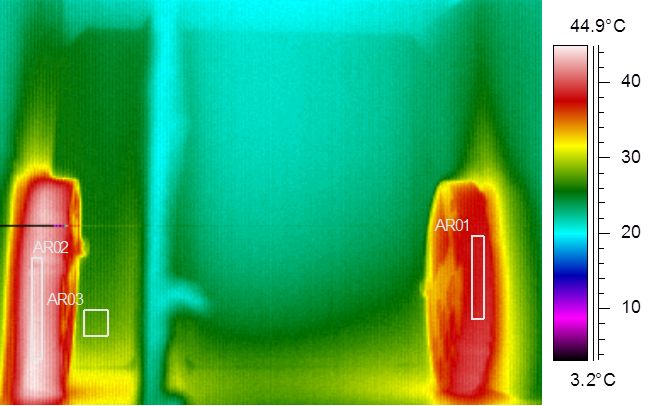
Note different shape of plate sense areas and AR03 sensing back wall temp on hot side

Synchronising to 120deg C at time 0 Absolute temperature  - note backwall temperatures now included

Synchronised to 120C diffenece between hot plate and warm plate and hot only setups

Resynchronising at 76degC at time zero Absolute temperature

Still get widening temperature gap showing coolingof a hot plate is slowed by a warm plate

So again these 2 runs analysed differently show that a cool object (warmer than background) can slow the cooling of a hot plate

----------------------------------------



Thoughts for a repeat:

Continuous monitoring of ambient temperature.

Enclose hot plate in box of constructed with thermal insulation with 2 sides of cling film (limits heat loss to mainly IR).

Put constant power into the hot plate (fixed voltage across a resistor) Measure temperature with thermocouple - set to approximately 80C when facing ambient.

With hot plate facing plate atambient temperature

Allow temperature to stabilise

Remove ambient plate (possibly now above ambient)

Replace with warm plate at 70C initially

Allow temperature to "stabilise" should rise then fall as the warm plate cools

Remove warm plate leaving side open to ambient. 

Allow temperature to stabilise
 

Possible problem is the not quite thermally transparent cling film. - as this heats it will begin radiating. 

Improvement suggestions?



What Affects DLWIR?

Using the same data source as before, the same parameter nulling gives this set of curves



This is the variation of DLWIR with day of the year (as before but low prob results retained)

This is absolute humidity effect - not linear

Interesting (night is disabled - no cloud information) but DLWIR is greater in mornings and evenings.  Why not midday?

Station Pressure - Possibly a problem with conversion between % hum and abs humidity causes this.

Linear effect with temperature as would be expected

Again a non linear relation with ULWIR

Wild errors are removed from the result by using the trimmean funcion disposing of 25% of highest and 25% lowest values.
Cloud values are measured using a visual light camera - hence no results will be returned for hours of darkness for this analysis.

===========UPDATE====================================================
Instrumentation
u/dlwir
PRECISION INFRARED RADIOMETER
Model PIR
The Precision Infrared Radiometer, Pyrgeometer, is intended for unidirectional operation in the measurement, separately, of incoming or outgoing terrestrial radiation as distinct from net long-wave flux. The PIR comprises a circular multi-junction wire-wound Eppley thermopile which has the ability to withstand severe mechanical vibration and shock. Its receiver is coated with Parson's black lacquer (non-wavelength selective absorption). Temperature compensation of detector response is incorporated. Radiation emitted by the detector in its corresponding orientation is automatically compensated, eliminating that portion of the signal. A battery voltage, precisely controlled by a thermistor which senses detector temperature continuously, is introduced into the principle electrical circuit.
Isolation of long-wave radiation from solar short-wave radiation in daytime is accomplished by using a silicone dome. The inner surface of this hemisphere has a vacuum-deposited interference filter with a transmission range of approximately 3.5 to 50 µm.
SPECIFICATIONS
Sensitivity: approx. 4 µV/Wm-2.
Impedance: approx. 700 Ohms.
Temperature Dependence: ±1% over ambient temperature range -20 to +40°C.
Linearity: ±1% from 0 to 700 Wm-2.
Response time: 2 seconds (1/e signal).
Cosine: better than 5%.
Mechanical Vibration: tested up to 20 g's without damage.
Calibration: blackbody reference.
Size: 5.75 inch diameter, 3.5 inches high.
Weight: 7 pounds.
Orientation: Performance is not affected by orientation or tilt.
-------------------------
This looks as if it is measuring the heating effect (thermopile) of radiation hitting the dome of the sensor (transmission 3.5 to 50um. The thermopile of course generates a voltage dependant on the temperature difference between one side and the other The non-dome side is not exposed to external radiation so no effect there. However, the nondome side temperature must be measured and compensated.
The instrument also compensates for its own generated IR.
No assumption of BB radiation is assumed. It is the ACTUAL heating effect of IR radiation of narrow or wide bandwith hitting the sensor that is the cause.

If the radiative "temperature" is less than the receiver temperature then the thermopile still measures - see series of posts about thermal imaging - the camera microbolometers sitting at 20+C shows temperatures down to -40C

======================================================================
Dry bulb temperature / wet bulb / relative humidity

HMP45C-L Specifications

• Supply Voltage: 12 Vdc nominal (typically powered by datalogger)
• Current Drain: ≤4 mA (active)
• Sensor Diameter: 2.5 cm (1 in.)
• Sensor Length: 25.4 cm (10 in.)
• Cable Diameter: 0.8 cm (0.3 in.)
• Weight: 0.27 kg (0.6 lb)

Relative Humidity

• Sensor: Vaisala’s HUMICAP® H-chip
• Measurement Range:
  0.8% to 100% RH, non-condensing
• Output Signal Range:
  0.008 to 1 Vdc
• Accuracy at 20°C (against factory reference): ±1% RH
• Accuracy at 20°C (field-calibrated against references):
  ±2% (0% to 90% RH);
  ±3% (90% to 100% RH)
• Temperature Dependence: ±0.05% RH/°C
• Long-Term Stability: Typically, better than 1% RH per year
• Response Time: 15 s with membrane filter (at 20°C, 90% response)
• Settling Time: 500 ms

Temperature

• Temperature Sensor: 1000 ohm Platinum Resistance Thermometer
• Measurement Range: -39.2° to +60°C
• Output Signal Range:
  0.008 to 1.0 V
• Accuracy:
  ±0.5°C (-40°C),
  ±0.4°C (-20°C),
  ±0.3°C (0°C),
  ±0.2°C (20°C),
  ±0.3°C (40°C),
  ±0.4°C (60°C)

====================================================================
Cloud - total and opaque

TSI-880 AUTOMATIC TOTAL SKY IMAGER

General Description The Total Sky Imager Model TSI-880 is an automatic, full-color sky imager system that provides real-time processing and display of daytime sky conditions. At many sites, the accurate determination of sky conditions is a highly desirable yet rarely attainable goal. Traditionally, human observers reported sky conditions, resulting in considerable discrepancies from subjective observations. In practice, the use of human observers is not always feasible due to budgetary constraints. The TSI-880 now replaces the need for these human observers under all weather conditions. An onboard processor computes both fractional cloud cover and sunshine duration, storing the results and presenting data to users via an easy-to-use web browser interface. The self-contained design makes it well suited for mission-critical applications such as aviation and military meteorology monitoring. It captures images into standard JPEG files that are analyzed into fractional cloud cover; if networked via TCP/IP (10/100BaseT) or PPP (modem) it becomes a sky image server to remote any user via the web. TSI-880 AUTOMATIC TOTAL SKY IMAGER General Description The Total Sky Imager Model TSI-880 is an automatic, full-color sky imager system that provides real-time processing and display of daytime sky conditions. At many sites, the accurate determination of sky conditions is a highly desirable yet rarely attainable goal. Traditionally, human observers reported sky conditions, resulting in considerable discrepancies from subjective observations. In practice, the use of human observers is not always feasible due to budgetary constraints. The TSI-880 now replaces the need for these human observers under all weather conditions. An onboard processor computes both fractional cloud cover and sunshine duration, storing the results and presenting data to users via an easy-to-use web browser interface. The self-contained design makes it well suited for mission-critical applications such as aviation and military meteorology monitoring. It captures images into standard JPEG files that are analyzed into fractional cloud cover; if networked via TCP/IP (10/100BaseT) or PPP (modem) it becomes a sky image server to remote any user via the web. Specifications Image Resolution: 352 x 288 color, 24-bit JPEG format Sampling rate: Variable, with max of 30 sec Operating Temperature: -40� C to +44� C Weight/Size: Approx.70 lbs.(32 kg); dims: 20.83"x18.78"; height is 34.19"; mounts on 16.75x12" 1/4-20 bolt square Power Requirements: 115/230 Vac; mirror heater duty cycle varies with air temperature: 560W with heater on / 60W off Software: None required for immediate real time display; uses Internet Explorer or Netscape Browsers on MS-Windows, Mac, UNIX (an optional DVE/YESDAQ package is available for data archiving, display, MPEG day movie creation and data reprocessing) Data Telemetry: LAN Ethernet (TCP/IP), telephone modem (PPP) or Data Storage Module option (for off grid sites) ==================================================================================== Precipitation: TE525-L Specifications Sensor Type: Tipping bucket/magnetic reed switch Material: Anodized aluminum Temperature: 0° to +50°C Resolution: 1 tip Volume per Tip: 0.16 fl. oz/tip (4.73 ml/tip) Rainfall per Tip: 0.01 in. (0.254 mm) Accuracy Up to 1 in./hr: ±1% 1 to 2 in./hr: +0, -3% 2 to 3 in./hr: +0, -5% Funnel Collector Diameter: 15.4 cm (6.06 in.) Height: 24.1 cm (9.5 in.) Tipping Bucket Weight: 0.9 kg (2.0 lb) ==================================================================================== Station Pressure CS105/CS105MD Barometric Pressure Sensor 1. General The CS105 analog barometer uses Vaisala’s Barocap silicon capacitive pressure sensor. The Barocap sensor has been designed for accurate and stable measurement of barometric pressure. The CS105 outputs a linear 0 to 2.5 VDC signal that corresponds to 600 to 1060 mb. It can be operated in a powerup or continuous mode. In the powerup mode the datalogger switches 12 VDC power to the barometer during the measurement. The datalogger then powers down the barometer between measurements to conserve power. 2. Specifications Operating Range Pressure: 600 mb to 1060 mb Temperature: -40 C to +60 C Humidity: non-condensing Accuracy Total Accuracy*** 0.5 mb @ +20 C 2 mb @ 0 C to +40 C 4 mb @ -20 C to +45 C 6 mb @ -40 C to +60 C Linearity*: 0.45 mb @ 20 C Hysteresis*: 0.05 mb @ 20 C Repeatability*: 0.05 mb @ 20 C Calibration uncertainty**: 0.15 mb @ 20 C Long-Term Stability: 0.1 mb per year * Defined as 2 standard deviation limits of end-point non-linearity, hysteresis error, or repeatability error ** Defined as 2 standard deviation limits of inaccuracy of the working standard at 1000 mb in comparison to international standards (NIST) *** Defined as the root sum of the squares (RSS) of end-point non-linearity, hysteresis error, repeatability error and calibration uncertainty at room temperature

Yearly CO2 variation Shown as Change in DLWIR?

Not sure about this post.
The data used is short
The data is noisy
Subtracting noisy signals does not improve accuracy!!

{UPDATE This data has now changed - I have nulled out the day of year changes and the long term variation(whole record) which significantly changes the results - the results will be posted at a later date]

Basically if CO2 is low then "back radiation" (DLWIR) should be lower than when CO2 is high
There is an annual cycly where CO2 dips in late spring and rises in autumn - see other posts.

So if you remove all factors changing downward long wave infrared radiation other than CO2 then what should be left is the yearly change in CO2 plus the long term increase.

The nulled data is inspected and a simple curve fit is applied and limits chosen that provide the best null for that factor.

Returned data that meets the criteria are averaged using a TRIMMEAN function to remove spurious high/low values

If the data is treated as a reapeated annual set then the long term becomes averaged and only the annual effect remains.

In the plots below the Nulled measurements are shown and CO2 at La Jolla is plotted for comparison.

The hourly measurement data is used

The analysis has been run many times each time there is always a dip starting at ~190 ( some ~60 days after the CO2 starts reducing)
Accuracy is nonsensical if less than 3 valid data are returned This unfortunately eliminates dec jan feb!.

However here are the final plots:

The raw data  (all points returning under 3 samples ignored) compared to La Jolla CO2

The smoothed data  (all points returning under 3 samples ignored) compare to La Jolla CO2

To pick sensible values for a number of variables the following limits are used.

Precipitation limit is set to eliminate any reading during "precipitation"
Cloud can only be measured during daylight
Only opaque cloud is considered
Humidity % is not used but is converted to absolute water vapour 

The Nulling Process

Each of the variables is nulled by plotting dlwir against the variable. Fitting a polynomial (order 1 to 6) to the resultant and then providing limits that deviate from the polynomial.  The polynomial is then applied to the extracted data.
Each variable is treated this way and then the process repeated until little change occurs. This produces the follwing limits.

start month	1
End month	12
hour min	11
hour max	15
Temp min	12.4
Temp max	29.4
Humidity Min	0
Humidity Max	1000
opaque Cloud Cover % min	2.8
opaque Cloud Cover % Max	30.9
cloud cover min	-999999
cloud cover max	1000
abs humid min	2.12
abs humid max	10.5
dlwir min	0
dlwir max	1000
ulwir min	445
ulwir max	595
dlwir as pc uplwir min	0
dlwir as pc uplwir max	100
start day	1
end day	19.2499
Pressure Min	809
Pressure Max	825
precipitation min	-1
precipitation Max	0.00001

These are the corrections applied:

	Temperature	opaque cld	ABS HUMIDITY	ULWIR	hour	Station pressure
x^6	-2.925607E-06	0.00E+00	0	0	0	0
x^5	4.16E-04	-1.30E-05	0	-1.73074E-09	0.01161075	0
x^4	-2.35E-02	1.05E-03	-0.01922243	4.37603E-06	-0.794129	0
x^3	6.78E-01	-3.04E-02	0.5449762	-0.004404108	21.56523	-0.001826181
x^2	-1.05E+01	3.83E-01	-5.604792	2.20558	-290.4116	4.45165
x	8.40E+01	-1.07E+00	29.91783	-549.6395	1938.646	-3617.085
c	3.22E+01	2.81E+02	108.4733	5.40E+04	-5133.338	979613.7

The nulling plots (not prettied up!)

Red plots are the result of nulling
blue lines are before nulling

Excel sheet is available (large)
Data is from (hourly):
http://www.nrel.gov/midc/srrl_bms/

Currently ~ 80,000 lines are analysed

Grape Harvest Temperature Reconstructions - More Stuff

Western European climate, and Pinot noir grape harvest dates in Burgundy, France, since the 17th century

http://www.int-res.com/articles/cr_oa/c046p243.pdf

from the document:

And something I did a few years ago.
Note the vertical scales are offset but per division scales are correct

And a comparison to CET

There seems to be no further analysis (more recent than 2003) which was done by:

 Chuine I, Yiou P, Viovy N, Seguin B, Daux V, Leroy Ladurie E (2004) Grape ripening as a past climate indicator.

From the above it seems that grapes despite possible  cultivar changes give a good proxy for temperature.

http://www.cefe.cnrs.fr/images/stories/DPTEFonctionnelle/BIOFLUX/Chercheurs/isabelle_chuine/publications/ChuineNature2004.pdf

http://www-ecole.enitab.fr/people/kees.vanleeuwen/articles/PI_36.pdf

Windmills - just no good? or more untruths in the press

The statements are mainly led by this document

http://www.ref.org.uk/attachments/article/280/ref.hughes.19.12.12.pdf

worthy of note is this blasting of prof hughes
https://s3.amazonaws.com/s3.documentcloud.org/documents/468709/imperial-college-supp-evidence-to-eec-wind.pdf

Nuclear and coal are often cited as always available
For example DRAX in uk is mentioned in bishops hill

But figures for recent availability (excludes time not required and not producing) come out at approx. 80%

Some plots using data from REFs own database

Each Turbine with approx 10 years record load factor plotted against year

A linear curve fit to Turbines output gives change in load factor per year

Note that the first graph shows all turbines load factor reducing until 2011 when a large recovery occurs. Is part of the loss caused by a reducing wind speed profile which then improves in 2011?

The second plot does show a general loss in efficiency over 10 years but nearer 7% total not the 15% suggested by Hughes document.

The REF site admits that 2010 was a low wind year:

"Overall, it is clear that the load factor for 2010 was low in comparison with preceding years, indicating that winds in this year, and particularly in the winter 2009-2010, were themselves relatively low."

There are 2 plots on the REF site:

http://www.ref.org.uk/publications/217-low-wind-power-output-2010
http://www.ref.org.uk/publications/229-renewables-output-in-2010

Note offset zero! If you ignore 2010 (low wind) the load factor looks pretty flat for the remaining 6 years

Offshore and onshore data combined?

Both plots from the owner of the daming report of Hughes show a different outcome to the reports conclusion.

2013-05-31
Diseases/disturbances reported by opponents:
http://tobacco.health.usyd.edu.au/assets/pdfs/publications/WindfarmDiseases.pdf
Well worth a read if you are looking for reasons to oppose the construction!

What DID happen to the ice during the Arctic Storm?

The daily rate of change is plotted below:

During the storm period 3 days show increased loss. Over the 2007 loss this is 292812 sq km

WUWT claim that this loss exposed more ice to later attack but only 2 other periods show gross changes:
During the period 15th August to 17th August (additional loss over 2007 is 178438 sq km)
During the period 22nd August to 23rd August (additional loss over 2007 is 174687 sq km)

So the Absolute maximum loss that could possibly be attributed to the "Great Arctic Storm" of 2012 is 645937 sq km.

The difference between the 2007 and 2012 minimum is 765468sq km

So even if you subtract the largest possible storm induced loss you would still have a 119531 sq km additional loss in 2012 when compared to 2007.

Sky Temperature and Thermal Imaging

Sky, High and Low cloud temperatures  as measured on a thermal imaging camera.

These images show the cloud and sky temperatures as measured by a camera with a 2µ to 13µ pass band.

From a previous test done at night the clear sky temperature is less than -40°C (the camera lower limit).

These pictures show that this clear sky value is maintained as expected during daylight (about -43°C).

Cloud temperatures range from -20°C for high light cloud to +1.1°C for low heavy cloud.

The pictures were taken on 21^st December 2012 at approx. 14:00pm  (sunset @ 16:00)
All area temperatures are maximum for that area.
 

 

 

 

These temperatures of course represent what the camera "sees" through its Germanium lense. And as can be seen from the previous thermal camera stuff the camera struggles to measure temperature of gasses - they just do not give black body radiation.

 

Previous posts:

http://climateandstuff.blogspot.co.uk/2012/12/water-vapour-and-thermal-imaging.html

http://climateandstuff.blogspot.co.uk/2012/11/thermal-imaging-how-not-to-measure.html

http://climateandstuff.blogspot.co.uk/2012/05/cool-body-can-transfer-measurable-heat.html

 

 



 

Water Vapour and Thermal imaging

More stuff about thermal imaging.

Looking at the sensitivity spectrum for a FLIR thermal camera much of the CO2 and H2O emission spectra are included but it is not a black body spectrum as the camera expects.

So does this mean that CO2 and water vapour should be less visible to the camera?

For the camera this is important since taking a photo through air which is emitting photons visible to its sensor would make its use limited – you would see the air not the object behind the air.

So a simple test using water vapour was done to see if this was the case

Some videos of a hot plate with 2 wells filled with water, The water is boiling but no hot vapour visible (vapour bubbles show approximately the expected temperature but the only vapour visible is less than 40°C.

If you now place a sheet of paper in the vapour the actual temperature of the vapour as it hits the paper can be seen (greater than 70°C)

Steam shows up at 28C

Shows paper being heated to 75.5C by steam invisible in gap between boiling water amd paper.

Heated plate showing 2 wells with boiling water

These videos show differen views of the hotplate - steam - paper system.

  

Steam visible + paper

Top view of plate, boiling water and paper

side view of plate boiling water and paper

Above videos seem to have problems  so a youtube version:

http://www.youtube.com/watch?feature=player_embedded&v=l3t9XeTIA1w

Conclusion: H2O vapour behaves as expected - despite the temperature being near boiling (100C) it does not appear so to the camera.

WUWT - cherry picking again

Water Vapour
The Watts nail in the coffin of AGW headline:

Another IPCC AR5 reviewer speaks out: no trend in global water vapor

Posted on December 14, 2012by Guest Blogger

New global water vapor findings contradict second draft of IPCC Assessment Report 5 (AR5)

Well, the paper this blogger / expert reviewer is behind a paywall so we have to assume that what he quotes is correct. But a quick search pulls up this paper

http://journals.ametsoc.org/doi/abs/10.1175/BAMS-86-2-245

This from the abstract TPW=total precipitable water:
...Further, we found out that the TPW anomalies are driven by the global surface temperature anomalies, but with a lag.

and from the text:

Time series plots of monthly and annual anomalies of TPW for the two datasets are shown in Figs. 8a and 8b, respectively. Also included in Fig. 8 is the global surface temperature anomaly, computed based on NASA’s Goddard Institute for Space Studies (GISS) global surface temperature data (Hansen et al. 1999).

The first 3 yr (1988–90) and part of 1996 show significant discrepancies between the anomalies of the two TPW datasets. There is, however, a good agreement for most parts of the other years. Linear regressionsbetween the two datasets show a correlation coefficient of 0.66 for the monthly anomalies and 0.74 for the annual anomalies. TPW anomalies are closely correlated to surface temperature anomalies. The correlation with surface temperature is higher for R-2 than for NVAP (Fig. 8d). The maximum cross correlation between TPW and surface temperature is reachedwhen the temperature leads the TPW by 2 months and equals 0.67 for R-2 and0.50 for NVAP. This suggests that precipitable water anomalies are driven by the temperature anomalies.

 

The problem is which cherry to pick?!!!!

 

 

Then of course Watts puts his foot in the wet and smelly with this blog post:

IPCC AR5 draft leaked, contains game-changing admission of enhanced solar forcing – as well as a lack of warming to match model projections, and reversal on ‘extreme weather’

Posted on December 13, 2012by Guest Blogger

So in this headline post we have a total misreading of a document. One of the authors  (and surely he should know) sais so on Australian Radio: .

The leaked IPCC drafts cover a range of subjects from the quality of climate models to measurements of sea level rise and Arctic ice loss.

Professor Steve Sherwood is a director of the Climate Change Research Centre at the University of New South Wales.

He is also a lead author of chapter seven of the IPCC report, which happens to be the one the sceptics are claiming for their side.

But Professor Sherwood is scornful of the idea that the chapter he helped write confirms a greater role for solar and other cosmic rays in global warming.

STEVE SHERWOOD: Oh that's completely ridiculous. I'm sure you could go and read those paragraphs yourself and the summary of it and see that we conclude exactly the opposite, that this cosmic ray effect that the paragraph is discussing appears to be negligible.

MARK COLVIN: They're saying that it is the first indication that the IPCC recognises something called solar forcing.

STEVE SHERWOOD: It's not the first time it recognises it. What it shows is that we looked at this. We look at everything. The IPCC has a very comprehensive process where we try to look at all the influences on climate and so we looked at this one.

And there have been a couple of papers suggesting that solar forcing affects climate through cosmic ray/cloud interactions, but most of the literature on this shows that that doesn't actually work.

MARK COLVIN: So you're saying that you've managed to basically eliminate this idea that sunspots or whatever are more responsible for global warming than human activity.

STEVE SHERWOOD: Based on the peer-reviewed literature that's available now, that looks extremely unlikely.

MARK COLVIN: So what have these people done? Is this just a case of cherry-picking a sentence?

STEVE SHERWOOD: Yeah, it's a pretty severe case of that, because even the sentence doesn't say what they say and certainly if you look at the context, we're really saying the opposite.

http://www.abc.net.au/pm/content/2012/s3654926.htm

It looks as if IPCC has played a blinder.

They can see where the "skeptics" will find inconsitancies and then clarify before publishing and all for free

They also show that sketics cannot read or comprehend!.

 

Cycle Mania and Hadcrut3

From the fun school of posts here are a couple of plots that reconstruct hadcrut3v from a series of sine waves.
One shows reconstruction from cycles only; this has problems getting a good fit in the 1800s but shows rhat the next few years should be a period of reducing temperatures. The long period controlling the plot is 317 year long
The other is constructed round a smooth increasing trend. A better fit in the 1800s and still shows that despite the trend the temperatures will be flat for a few more years before increasing with a vengance. The underlying trend is defined by this polynomial
y = 2.40389E-07x3 - 1.34093E-03x2 + 2.49320E+00x - 1.545547E+03

Do either have any predictive skills. = NO

The most importasnt thing shown is in the the trending plot where  despite an ever increasing trend there is still a period where temperatures appear not to increase - from 1998 to 2018. this is due to an underlying 60year period being on a down part of the cycle. This is something that the "skeptics" cannot seem to grasp - CO2 is increasing so why is temperature static?.

The all cycle:

317 year and 60.1 year cycles controlling the "trend"

The trend+cycle plot

Trend and 59.75 year cycle controlling trend

So what curve are we "following" - only another 4 or so years will tell!.

Earlier posts:
http://climateandstuff.blogspot.co.uk/search/label/simulation

Thermal Imaging - How Not to Measure Temperature

Thermal imaging cameras offer amazing perfomance - The one used here is accurate to +-2K and will discriminate temperatrue differences of as low as 0.08K.

However it seems that not many people realise they have limitations:
You cannot just point one at a subject and say what the temperature is. In some cases it is not possible to even guess the temperature of the object (reflective surface).

Here are some indications of what can go wrong.
A copper heatsink 3mm thick with various surface finishes is used to show the pitfalls:

One end of the matt tinplated copper block was polished until pure copper was exposed

The centre of the block was polished untill the tin plate was still present.

The plate was then spray painted down one half with matt grey paint.

First a video showing reflection from the unpainted side of a hot object moving

A still from the video

:

Now a video of the WHOLE of the plate heating :





Is the temperature of the block 23 26 or 41C?

 

 Note that the painted area shows insignificant change to the temperature whereas the unpainted side shows a reflection causing the reported temperature to change by approximately 20C

Next observe the plate being heated by electronics attached to the other side.
You will see the painted area slowly heating whils the bare metal changes very little: 

Finally Just to prove that the shiny side has not been masked Plate is hot and shiny side reflects hot object

How good is the grey undercoat at normalising the emissivity These 2 plots show how the temperature changes along the line LI01 placed first in the unpainted area and then in the painted area.:

With no paint this is the response of the plate

Painted - not perfect but a lot better.

So just what is the temperature of the plate? The answer is I do not know - it is approximately the temperature shown on the grey painted area... but since I have not calibrated the emissivity of the paint I do not know! And since I have not measured the humidity I do not know. And since I did not measure the distance from sensor to object I do not know. And since I did not measure the air temperature I do not know.

How about outside - NOTE these are not calibrated images no emissivity/atmospheric corrections applied.
Time taken 2012-11-14 17:45  Ambient temperature 7.0C Camera range -40 to 120C hence some of the temperatures measured are outside the camera range (-45C seems to be the saturation level of measurement). Humidity ? high

So it seems that clear sky no sun has a "temperature" of about -44C and seems to decrease linearly with angle above the horizon.

Take a picture of a MMT thermometer and claim that the temperature of the case is X is wrong unless you have eliminated reflections and calibrated the emissivity.

Take temperatures of houses and you will show heat leaks and hot spots but you cannot claim that the temperature has much accuracy (it will be more accurate than the shiny MMT surface)

What is interesting is of course that you can take thermal images through the atmosphere. This proves there is little emissions in the thermal IR band from resident gases.

The IR spectrum (from FLIR documentation):

 FLIR S45 camera Spectral Range 7.5 to 13um

Germanium used for lens has this transmission vs wavelength property:

Beware of what you read at WUWT!

see also this post:
http://climateandstuff.blogspot.co.uk/2012/05/cool-body-can-transfer-measurable-heat.html