Showing posts with label co2. Show all posts

2013/02/09

What Affects DLWIR?

Using the same data source as before, the same parameter nulling gives this set of curves


This is the variation of DLWIR with day of the year (as before but low prob results retained)

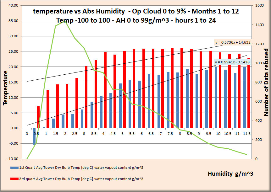
This is absolute humidity effect - not linear

Interesting (night is disabled - no cloud information) but DLWIR is greater in mornings and evenings.  Why not midday?

Station Pressure - Possibly a problem with conversion between % hum and abs humidity causes this.

Linear effect with temperature as would be expected

Again a non linear relation with ULWIR
Wild errors are removed from the result by using the trimmean funcion disposing of 25% of highest and 25% lowest values.
Cloud values are measured using a visual light camera - hence no results will be returned for hours of darkness for this analysis.

===========UPDATE====================================================
Instrumentation
u/dlwir
PRECISION INFRARED RADIOMETER
Model PIR
The Precision Infrared Radiometer, Pyrgeometer, is intended for unidirectional operation in the measurement, separately, of incoming or outgoing terrestrial radiation as distinct from net long-wave flux. The PIR comprises a circular multi-junction wire-wound Eppley thermopile which has the ability to withstand severe mechanical vibration and shock. Its receiver is coated with Parson's black lacquer (non-wavelength selective absorption). Temperature compensation of detector response is incorporated. Radiation emitted by the detector in its corresponding orientation is automatically compensated, eliminating that portion of the signal. A battery voltage, precisely controlled by a thermistor which senses detector temperature continuously, is introduced into the principle electrical circuit.
Isolation of long-wave radiation from solar short-wave radiation in daytime is accomplished by using a silicone dome. The inner surface of this hemisphere has a vacuum-deposited interference filter with a transmission range of approximately 3.5 to 50 µm.
SPECIFICATIONS
Sensitivity: approx. 4 µV/Wm-2.
Impedance: approx. 700 Ohms.
Temperature Dependence: ±1% over ambient temperature range -20 to +40°C.
Linearity: ±1% from 0 to 700 Wm-2.
Response time: 2 seconds (1/e signal).
Cosine: better than 5%.
Mechanical Vibration: tested up to 20 g's without damage.
Calibration: blackbody reference.
Size: 5.75 inch diameter, 3.5 inches high.
Weight: 7 pounds.
Orientation: Performance is not affected by orientation or tilt.
-------------------------
This looks as if it is measuring the heating effect (thermopile) of radiation hitting the dome of the sensor (transmission 3.5 to 50um. The thermopile of course generates a voltage dependant on the temperature difference between one side and the other The non-dome side is not exposed to external radiation so no effect there. However, the nondome side temperature must be measured and compensated.
The instrument also compensates for its own generated IR.
No assumption of BB radiation is assumed. It is the ACTUAL heating effect of IR radiation of narrow or wide bandwith hitting the sensor that is the cause.

If the radiative "temperature" is less than the receiver temperature then the thermopile still measures - see series of posts about thermal imaging - the camera microbolometers sitting at 20+C shows temperatures down to -40C

======================================================================
Dry bulb temperature / wet bulb / relative humidity

HMP45C-L Specifications

  • Supply Voltage: 12 Vdc nominal (typically powered by datalogger)
  • Current Drain: ≤4 mA (active)
  • Sensor Diameter: 2.5 cm (1 in.)
  • Sensor Length: 25.4 cm (10 in.)
  • Cable Diameter: 0.8 cm (0.3 in.)
  • Weight: 0.27 kg (0.6 lb)

Relative Humidity

  • Sensor: Vaisala’s HUMICAP® H-chip
  • Measurement Range:
    0.8% to 100% RH, non-condensing
  • Output Signal Range:
    0.008 to 1 Vdc
  • Accuracy at 20°C (against factory reference): ±1% RH
  • Accuracy at 20°C (field-calibrated against references):
    ±2% (0% to 90% RH);
    ±3% (90% to 100% RH)
  • Temperature Dependence: ±0.05% RH/°C
  • Long-Term Stability: Typically, better than 1% RH per year
  • Response Time: 15 s with membrane filter (at 20°C, 90% response)
  • Settling Time: 500 ms

Temperature

  • Temperature Sensor: 1000 ohm Platinum Resistance Thermometer
  • Measurement Range: -39.2° to +60°C
  • Output Signal Range:
    0.008 to 1.0 V
  • Accuracy:
    ±0.5°C (-40°C),
    ±0.4°C (-20°C),
    ±0.3°C (0°C),
    ±0.2°C (20°C),
    ±0.3°C (40°C),
    ±0.4°C (60°C)
====================================================================
Cloud - total and opaque

TSI-880 AUTOMATIC TOTAL SKY IMAGER

General Description The Total Sky Imager Model TSI-880 is an automatic, full-color sky imager system that provides real-time processing and display of daytime sky conditions. At many sites, the accurate determination of sky conditions is a highly desirable yet rarely attainable goal. Traditionally, human observers reported sky conditions, resulting in considerable discrepancies from subjective observations. In practice, the use of human observers is not always feasible due to budgetary constraints. The TSI-880 now replaces the need for these human observers under all weather conditions.
An onboard processor computes both fractional cloud cover and sunshine duration, storing the results and presenting data to users via an easy-to-use web browser interface. The self-contained design makes it well suited for mission-critical applications such as aviation and military meteorology monitoring. It captures images into standard JPEG files that are analyzed into fractional cloud cover; if networked via TCP/IP (10/100BaseT) or PPP (modem) it becomes a sky image server to remote any user via the web.
Specifications

Image Resolution: 352 x 288 color, 24-bit JPEG format
Sampling rate: Variable, with max of 30 sec
Operating Temperature: -40 C to +44 C
Weight/Size: Approx.70 lbs.(32 kg); dims: 20.83"x18.78"; height is 34.19"; mounts on 16.75x12" 1/4-20 bolt square
Power Requirements: 115/230 Vac; mirror heater duty cycle varies with air temperature: 560W with heater on / 60W off
Software: None required for immediate real time display; uses Internet Explorer or Netscape Browsers on MS-Windows, Mac, UNIX (an optional DVE/YESDAQ package is available for data archiving, display, MPEG day movie creation and data reprocessing)
Data Telemetry: LAN Ethernet (TCP/IP), telephone modem (PPP) or Data Storage Module option (for off grid sites)
====================================================================================
Precipitation:

TE525-L Specifications

  • Sensor Type: Tipping bucket/magnetic reed switch
  • Material: Anodized aluminum
  • Temperature: 0° to +50°C
  • Resolution: 1 tip
  • Volume per Tip: 0.16 fl. oz/tip (4.73 ml/tip)
  • Rainfall per Tip: 0.01 in. (0.254 mm)
  • Accuracy
    Up to 1 in./hr: ±1%
    1 to 2 in./hr: +0, -3%
    2 to 3 in./hr: +0, -5%
  • Funnel Collector Diameter:
    15.4 cm (6.06 in.)
  • Height: 24.1 cm (9.5 in.)
  • Tipping Bucket Weight:
    0.9 kg (2.0 lb)
====================================================================================
Station Pressure

CS105/CS105MD Barometric Pressure
Sensor
1. General
The CS105 analog barometer uses Vaisala’s Barocap silicon capacitive
pressure sensor. The Barocap sensor has been designed for accurate and stable
measurement of barometric pressure. The CS105 outputs a linear 0 to 2.5
VDC signal that corresponds to 600 to 1060 mb. It can be operated in a
powerup or continuous mode. In the powerup mode the datalogger switches
12 VDC power to the barometer during the measurement. The datalogger then
powers down the barometer between measurements to conserve power.
2. Specifications
Operating Range
Pressure: 600 mb to 1060 mb
Temperature: -40 C to +60 C
Humidity: non-condensing
Accuracy
Total Accuracy*** 0.5 mb @ +20 C
2 mb @ 0 C to +40 C
4 mb @ -20 C to +45 C
6 mb @ -40 C to +60 C
Linearity*: 0.45 mb @ 20 C
Hysteresis*: 0.05 mb @ 20 C
Repeatability*: 0.05 mb @ 20 C
Calibration uncertainty**: 0.15 mb @ 20 C
Long-Term Stability: 0.1 mb per year
* Defined as 2 standard deviation limits of end-point non-linearity,
hysteresis error, or repeatability error
** Defined as 2 standard deviation limits of inaccuracy of the working
standard at 1000 mb in comparison to international standards (NIST)
*** Defined as the root sum of the squares (RSS) of end-point non-linearity,
hysteresis error, repeatability error and calibration uncertainty at room
temperature


2013/01/20

Yearly CO2 variation Shown as Change in DLWIR?

Not sure about this post.
The data used is short
The data is noisy
Subtracting noisy signals does not improve accuracy!!

{UPDATE This data has now changed - I have nulled out the day of year changes and the long term variation(whole record) which significantly changes the results - the results will be posted at a later date]

Basically if CO2 is low then "back radiation" (DLWIR) should be lower than when CO2 is high
There is an annual cycly where CO2 dips in late spring and rises in autumn - see other posts.

So if you remove all factors changing downward long wave infrared radiation other than CO2 then what should be left is the yearly change in CO2 plus the long term increase.

The nulled data is inspected and a simple curve fit is applied and limits chosen that provide the best null for that factor.

Returned data that meets the criteria are averaged using a TRIMMEAN function to remove spurious high/low values

If the data is treated as a reapeated annual set then the long term becomes averaged and only the annual effect remains.

In the plots below the Nulled measurements are shown and CO2 at La Jolla is plotted for comparison.

The hourly measurement data is used

The analysis has been run many times each time there is always a dip starting at ~190 ( some ~60 days after the CO2 starts reducing)
Accuracy is nonsensical if less than 3 valid data are returned This unfortunately eliminates dec jan feb!.

However here are the final plots:
The raw data  (all points returning under 3 samples ignored) compared to La Jolla CO2

The smoothed data  (all points returning under 3 samples ignored) compare to La Jolla CO2
To pick sensible values for a number of variables the following limits are used.

Precipitation limit is set to eliminate any reading during "precipitation"
Cloud can only be measured during daylight
Only opaque cloud is considered
Humidity % is not used but is converted to absolute water vapour 

The Nulling Process

Each of the variables is nulled by plotting dlwir against the variable. Fitting a polynomial (order 1 to 6) to the resultant and then providing limits that deviate from the polynomial.  The polynomial is then applied to the extracted data.
Each variable is treated this way and then the process repeated until little change occurs. This produces the follwing limits.

start month1
End month12
hour min11
hour max15
Temp min12.4
Temp max29.4
Humidity Min0
Humidity Max1000
opaque Cloud Cover % min2.8
opaque Cloud Cover % Max30.9
cloud cover min-999999
cloud cover max 1000
abs humid min2.12
abs humid max10.5
dlwir min0
dlwir max1000
ulwir min445
ulwir max595
dlwir as pc uplwir min0
dlwir as pc uplwir max100
start day1
end day19.2499
Pressure Min809
Pressure Max825
precipitation min-1
precipitation Max0.00001

These are the corrections applied:

Temperature opaque cldABS HUMIDITYULWIRhourStation pressure
x^6-2.925607E-060.00E+000000
x^54.16E-04-1.30E-050-1.73074E-090.011610750
x^4-2.35E-021.05E-03-0.019222434.37603E-06-0.7941290
x^36.78E-01-3.04E-020.5449762-0.00440410821.56523-0.001826181
x^2-1.05E+013.83E-01-5.6047922.20558-290.41164.45165
x8.40E+01-1.07E+0029.91783-549.63951938.646-3617.085
c3.22E+012.81E+02108.47335.40E+04-5133.338979613.7

The nulling plots (not prettied up!)


Red plots are the result of nulling
blue lines are before nulling

Excel sheet is available (large)
Data is from (hourly):
http://www.nrel.gov/midc/srrl_bms/

Currently ~ 80,000 lines are analysed


2012/06/14

Further thoughts on CO2 Cycle

Found some O2 data for Alert Alaska. Plotting this on the same graph as Barrow give the plot below.
This shows that O2 is the inverse of CO2 with the peak of O2 occurring (as near as can be determined from the sparse data) at the minimum of CO2. They appear to be in synchronism.

To me this shows that the O2 and CO2 are linked to the same process.


From http://www.elcamino.edu/faculty/tnoyes/Readings/10AR.pdf this plot shows that there is a peak phytoplankton growth in summer at the poles which is significantly higher than spring or autumn growths.

Phytoplankton in sunlight photosynthesises using CO2 and creating O2. In the dark O2 is used in phytoplankton respiration and CO2 is released.

Decomposition requires warm temperatures for the bacteria to work.At the end of summer temperatures are falling rapidly so decomposition will not release CO2 rapidly and certainly would not continue into December. This suggests that spring growth and autumn decomposition would not cause the CO2 dip.

Conclusion:
The CO2 dip is caused by the action of sunlight on phytoplankton.


The Full O2 record with CO2

2012/06/08

CO2 cycle revisited

A previous post had a look at the CO2 cycle and questioned the cause.
This post adds a couple more years of data but still does not solve the dip cause.

Latest Data Showing the approx dip measurement points:


Depth of dip replotted.


Note the innaccuracy of determining the depth gives a different plot to the last investigation.

The cause?

Ice covering phyto plankton - as more is exposed to sunlight photosynthesis overcomes respiration and co2 is absorbed from the sea wich then absorbs it from the air.

http://www.ldeo.columbia.edu/~marra/PhytoRespGRLv5.pdf

Change at equinox considering respiration/photosynthesis in phytoplankton and plants
Daylight time is greater than dark time prior to 22nd September and less than dark after this date? Trouble is the dip is around the end of August and the 1st week in September.
Why should the dip be earlier?

Growth/decay of land plants
Growth - ok CO2 is converted to biomass
Decay - much too slow over the winter months to return the CO2

Water temperature.
Warm water takes up less CO2 than cold so is wrong direction for dip.


Most likely
 equinox and length of day/night affecting the respiration/photosynthesis balance?
Depth of dip is greatest at Barrow and gets smaller the further south you go. Eventually the phase of the dip changes as you would expect for the southern hemisphere.


Still no further forward!

2012/05/27

The Complex World of Humidity and Temperature

During sunlight hours (minimal cloud) the water vapour in the air will absorb long wave IR (Green House Effect) from the sun and from the ground.
This will be radiated back in all directions.
The solar radiation will therefore be modified such that the wavelengths absorbed by the water vapour will be reduced depending on the effectiveness of the green house effect.
 However the same wavelengths radiated upwards will be more effectively "reflected" back down.

At night the solar input stops and the only radiation hitting the earth is that from GHGs So more water vapour = better "reflector"

Is this visible in the data previously used below.
Firstly data is limited and to get sensible results each point needs significantly more than one result to be significant.

Night time readings cannot include cloud coverage as this is not measured when dark
The former plots used either average or min/max values. The min max tend to plot one off anomalies. In the plots below 1st and 3rd quartile results have been used to improve this.

First a whole year all possible times with up to 9% opaque cloud cover

http://www.nrel.gov/midc/srrl_bms/

not sure why humidity so high!
Now in sequence 2 months at a time a couple of hours and up to 9% opaque cloud cover
Now for some night responses 2 months at a time
Conclusion?

  • Well minimum temperature shows a increase with increasing water vapour (positive slope) over coldest period but turns to negative slope during warmer months
  • The max temp during the night shows little change with water vapour.


2012/04/21

DLWIR Holding 2 parameters at the limit allowing sensible results

A couple of re-plots with less variation in the 2 other params. Also added a count of returned results for each measurement

Basically More cloud = less escaping radiation - not a lot of difference between total and opaque cloud coverage

But the biggest effect is from water vapour. With the small number of samples it looks as if the response is logarithmic with percentage relative humidity.


2012/04/16

Backradiation - fixing the effect of 2 variables plotting the third

Up to now I've plotted the effect of cloud coverage, humidity and temperature on the difference between DLWIR and ULWIR.

However these plots are not a simple xy since there may be a correlation between temperature/humidity and clouds.

To improve the plots it would be best to plot for example humidity vs dlwir/ulwir at a fixed temperature and cloud cover. The problem is there are too few corresponding points to get a meaningful result.

The following plots were made by inspecting plots and choosing a range of values for each parameter where the dlwir/ulwir change is minimal (about 10% or less)

As a trial cloud coverage was replotted at a much closer variation in the other 2 parameters - this shows a good correspondance with the wider variation but with increased variability.

It should be pointed out that the dlwir as a % of ulwir is a combination of at least all the 3 parameters considered. All that can be gleaned from these plots is the effect of variation of  one parameter whilst holding the others static.

It should be noted that cloud cover is only measured during daylight. All the plots below are therefore only relevant for daylight.


From the above it can be seen that the:

temperature effect is inconsistent and small
relative humidity is the largest effect - more humidity more DLWIR
Cloud cover is significant - more clouds more DLWIR


2012/04/15

The Effect of Humidity on Back Radiation

Continuing the same theme Here is the effect of changing Humidity (both relative and absolute) on the percentage of backradiation compared to upward radiation


Difficult finding a conversion between relative humidity (as measured) and absolute humidity.
the equation used for the above plot was:
abs humidity=1320.65/(273+T)*rh/100*10^(7.4475*(T+273-273.14)/(T+273-39.44))


So It looks as if the effects of cloud cover / temperature should only be made at fixed RH.

Yet more sums to do!

2012/01/02

Are Adiabatic Lapse Rates Controlling Temperatures

Better stuff here on adiabatic lapse rates!!
http://scienceofdoom.com/2012/08/12/temperature-profile-in-the-atmosphere-the-lapse-rate/

Some of the rest is interesyting in this post:


Adiabatic Lapse Rates
wiki
Types of lapse rates

There are two types of lapse rate:
 Environmental lapse rate – which refers to the actual change of temperature with altitude for the stationary atmosphere (i.e. the temperature gradient)
 The adiabatic lapse rates – which refer to the change in temperature of a parcel of air as it moves upwards (or downwards) without exchanging heat with its surroundings. The temperature change that occurs within the air parcel reflects the adjusting balance between potential energy and kinetic energy of the molecules of gas that comprise the moving air mass. There are two adiabatic rates:[6] Dry adiabatic lapse rate
 Moist (or saturated) adiabatic lapse rate
http://www4.uwsp.edu/geO/faculty/ritter/geog101/textbook/atmospheric_moisture/lapse_rates_1.html
In "The Atmosphere" we discovered that air temperature usually decreases with an increase in elevation through the troposphere. The decrease in temperature with elevation is called the environmental lapse rate of temperature or normal lapse rate of temperature. Recall that  the normal lapse rate of temperature is the average lapse rate of temperature of .65o C / 100 meters. The environmental lapse rate of temperature is the actual vertical change in temperature on any given day and can be greater or less than .65o C / 100 meters.  Also recall that the decrease in temperature with height is caused by increasing distance from the source of energy that heats the air, the Earth's surface. Air is warmer near the surface because it's closer to its source of heat. The further away from the surface, the cooler the air will be. It's like standing next to a fire, the closer you are the warmer you'll feel. Temperature change caused by an exchange of heat between two bodies is called diabatic temperature change. There is another very important way to change the temperature of air called adiabatic temperature change.
 http://daphne.palomar.edu/jthorngren/adiabatic_processes.htm
Make sure you notice that we are talking about moving air (rising or subsiding),  not still air.  The change in temperature of still air (that is, air that is not rising or subsiding) follows the Environmental Lapse  Rate, which varies considerably, but averages about 6.5 deg C/1000 meters  (3.6 deg/1000 feet).  In still air, if you went up in a hot air balloon, carrying a thermometer and taking the air temperature every 1000 meters, on average the temperature would drop 6.5 degrees C every 1000 meters.  The rate of temperature change as you rise in still air is not as great as the rate of change of rising air; that is, the air parcel does not cool off as fast.
For instance, the air temperature at sea level is 28 degrees C.  Climb into your balloon, release the tethers, and go up 1000 meters in the still air.  On average, the air temperature 1000 meters up will be _21.5___degrees C.   If the air were rising, and the temperature at sea level was 28 degrees C, what would the temperature of the air be after it rose 1000 meters? 18C
http://www.sci.uidaho.edu/scripter/geog100/lect/05-atmos-water-wx/05-part-7-atmos-lifting-fronts/ch5-part-7a-atmos-liftin.htm
http://www.geographypages.co.uk/lapse.htm
http://www.st-andrews.ac.uk/~dib2/climate/lapserates.html
People talk of adiabatit lapse rates as if they control the atmosperic temperatre. Why?
These lapse rates refer to moving a number of molecules from low pressure to high pressure and getting heated. No problem with that. BUT
For every molecule moved down to high press ure there must be a molecule moved from high to low. It cannot be a one way transport (obviously!).
So, in my books, the heating effect of falling molecules equals the cooling effect of rising molecules. Hence no effect.
So Why is it colder up a mountain than on the plains.
GHG free air absorbs litle of the available sunlight. Air with GHGs absorbs only at the known absoption frequencies and the proportion of theses frequencies in the TSI is relatively small. There is therefore little air heating due to sunlight.
However sunlight hits the ground and 70% gets absorbed and reradiated as heat at long wave infra red frequencies. These will heat the air via absoption. There is more close ground creating warming in a valley than on a hill hence it will be warmer.
NOW if there is a 1000 metre plateau will this be as warm as the valley below - if not, why not?

from WUWT
The adiabatic lapse rate is defined by the "gas Laws" not by gravity (other than of course high gravity gives high pressure!).
The adiabatic lapse rate requires that a fixed number of molecules be moved between pressure differences. Once at a new pressure the new temperature will stabilise to the surroundings (but that is not what adiabatic lapse rate is about).
However, for every molecule transported from high to low pressure there MUST be a molecule transported from low to high pressure. This means there is NO net flow of energy.
Where the atmosphere blends into a vacuum there can be no convective/conductive transfer of energy (there is nothing to transfer the energy to!)
Radiation is the only option. N2 H2 O2 etc. have little propensity to absorb radiation. Hoever they will get warm by transfer of heat from GH gasses. All hot bodies emit radiation (bb radiation).

At the other end of the air column you have similar problems. The ground/sea warms through absorption of the shorter wavelengths of TSI (where most of the solar energy is). The heat is radiated from the ground/sea as LWIR and by contact at the boundary between earth and atmosphere. The heat must be transferred from molecule to molecule by contact or by convection. A slow process. Conduction will be enhanced by high pressure, convection will be slowed.
The radiated energy is NOT significantly absorbed by O2 N2 H2 etc. no matter what the pressure. Even a solid glass fibre can be made extremely low loss 0.2dB per km and the molecules are pretty solidly packed http://www.fiberoptics4sale.com/wordpress/optical-fiber-loss-and-attenuation/ . Without a GHG this radiation would escape without attenuation straight to space. GHGs will "absorb" this LWIR at certain frequencies and re-emit it in all directions. The time for this energy to be "reabsorbed" in another molecule is dependent on the path length which is dependent on the proximity of other GHG molecules which is dependant on the pressure of the atmosphere.
The time taken for the radiation to bounce from molecule to molecule increases the time it takes for the energy to travel from ground to space.
The energy input to the system is at a constant rate. Slow down the output and the system gets hotter. A hotter system will radiate more energy (BB radiation).
Where does the energy from static pressure difference come in to this?


Atmospheric longwave irradiance uncertainty: Pyrgeometers compared to an absolute sky-scanning radiometer, atmospheric emitted radiance interferometer, and radiative transfer model calculations.


================
Downward longwave irradiance uncertainty under arctic atmospheres: Measurements and modeling
http://www.slf.ch/ueber/mitarbeiter/homepages/marty/publications/Marty2003_IPASRCII_JGR.pdf
Figure 2

Spectral and Broadband Longwave Downwelling Radiative Fluxes, Cloud Radiative

Forcing, and Fractional Cloud Cover over the South Pole
http://www.webpages.uidaho.edu/~vonw/pubs/TownEtAl_2005.pdf


Measurement of night time downward radiation
So we know the solar output received in the dark is 0
We know that O2 and N2 have very very very little thermal radiation.
So where does all that downward radiation come from (at least 270W/sqm)
It can only be from GHGs.
During the day we receive about 380W/sqm
So the 270W/sqm is additional to the solar irradiance.
So the average night day temp difference is less than expected (no sideways conduction/wind required)
N2 O2 absoptions are mainly rotational and thereefore mainly in the microwave region. There is not a great amount of radiation in these frequencies.

Cloud transmission (from above-FTIR looking down) from
An introduction to atmospheric radiation
By Kuo-Nan Liou


Transmission through the atmosphere. If GH effect exists then there should be mmissing parts of emission spectrum when looking at the earth. AND when looking up at the sky there should be higher levels of radiation at the same wavelengt as is missing when looking down. Is this the case? It seems so:


spectral plot is here:
http://www.patarnott.com/atms749/powerpoint/ch6_GP.ppt

IR great plains measured here:
SGP Central Facility, Ponca City, OK
36° 36' 18.0" N, 97° 29' 6.0" W
Altitude: 320 meters
http://www.arm.gov/sites/sgp

Better stuff here!!
http://scienceofdoom.com/2012/08/12/temperature-profile-in-the-atmosphere-the-lapse-rate/


2011/02/25

A Plot to remember. A post to remember. A Writ to remember.


Absolute garbage concatenation of two approximations ignoring continental movements.
The temperature to me seems to show warm/cold/not so warm type of temperatures not that it was 25C 600M years ago!
http://www.scotese.com/climate.htm
The CO2 comes from a MODEL described here
http://earth.geology.yale.edu/~ajs/2001/Feb/qn020100182.pdf

Its snowing CO2 in the antarctic!!
http://wattsupwiththat.com/2009/06/09/co2-condensation-in-antarctica-at-113f/


The original title:
Natural Carbon Sequestration In Antarctica ? A Litmus Test For Global Warming? By Steven Goddard How cold is it in Antarctica? According to Weather Underground, Vostok, Antarctica is forecast to reach -113F on Friday. That is four degrees below the freezing point of CO2 and would cause dry (CO2) ice to freeze directly out of the air.

added 18/1/2013


Cuccinelli vs UVA
http://s3.amazonaws.com/hamptonroadscom/store/1611.pdf

he wants even the used toilet paper!

Definition of document
"any book, pamphlet, brochure, periodical, newspaper, letter, correspondence, memoranda, notice, facsimile, e-mail, manual, press release, telegram, report, study, handwritten note, working paper, chart, paper, graph, index, tape, data processingcard,, or any otherwritten, recorded, transcribed, punched, taped, filmed, or graphic matter now in your possession, custody, or control"

2010/11/25

Watts - More garbage

The latest watts misinformation and all over a picture:


Watts contention starts out as being the data is false in the background information.
Watts' telling comment is
Huh, that’s strange, it only shows around 280ppm of CO2 at the “present” of 1999 when this graph was published
 
The trouble is he has forgotten that present in general refers to 1950 in ice core timelines
The vostock Ice core finishes 2400 years before present (1950) i.e. some 500 years BC.


Then watts goes on to complain that the real problem is splicing valid CO2 readings  from the present to paleo data,

 But CO2 is a well mixed gas over the globe
Now here’s the problem. If you took surface temperature data from Antarctica, and spliced it with surface temperature data from Hawaii, and then presented it as the entire historical record from Antarctica, our friends would have a veritable “cow”.


This shows most of the CO2 records fall within +-1ppm with a couple of outliers at +-5ppm (linear) looking at the monthly plots shows that the peak at alert Alaska occurs some 2 months before the peak at Mauna Loa. Indicating that CO2 is pretty much in synch.

Yes, I agree that a spliced data should be indicated (perhaps the previous slide showed just the vostok data and was then compared to current data in the slide used as background???) But there is no invalid information in the picture.

2010/02/19

CO2 saturation

An understandable explanation of CO2 and how it will not saturate:

"So, if a skeptical friend hits you with the "saturation argument" against global warming, here’s all you need to say: (a) You’d still get an increase in greenhouse warming even if the atmosphere were saturated, because it’s the absorption in the thin upper atmosphere (which is unsaturated) that counts (b) It’s not even true that the atmosphere is actually saturated with respect to absorption by CO2, (c) Water vapor doesn’t overwhelm the effects of CO2 because there’s little water vapor in the high, cold regions from which infrared escapes, and at the low pressures there water vapor absorption is like a leaky sieve, which would let a lot more radiation through were it not for CO2, and (d) These issues were satisfactorily addressed by physicists 50 years ago, and the necessary physics is included in all climate models"

http://www.realclimate.org/index.php/archives/2007/06/a-saturated-gassy-argument/
http://www.realclimate.org/index.php/archives/2007/06/a-saturated-gassy-argument-part-ii/

2009/11/09

CO2 the stuff of life

Lets look at 2 gases
a poison – Hydrogen Sulphide H2S
And a benificial to all life nutrient – CO2

H2S
http://www.drthrasher.org/toxicology_of_hydrogen_sulfide.html
10 ppm
Beginning of Eye Irritation
50-100 ppm
Slight conjunctivitis and respiratory tract irritation after one hour
100 ppm
Coughing, eye irritation, loss of sense of smell after 2-15 minutes. Altered respiration, pain the eyes, and drowsiness after 15-30 minutes followed by throat irritation after one hour. Several hours exposure results in gradual increase in severity of symptoms and death may occur within the next 48 hours.
200-300 ppm
Marked conjunctivitis and respiratory tract irritation after one hour exposure.
500-700 ppm
Loss of consciousness and possibly death in 30 minutes to one hour of exposure.
700-1000 ppm
Rapid unconsciousness, cessation of respiration, and death
1000-2000 ppm
Unconsciousness at once, with early cessation of respiration and death in a few minutes. Death may occur if individual is removed to fresh air at once.

The most dangerous aspect of hydrogen sulfide results from olfactory accomodation and/or olfactory paralysis. This means that the individual can accomodate to the odor and is not able to detect the presence of the chemical after a short period of time. Olfactory paralysis occurs in workers who are exposed to 150 ppm or greater. This occurs rapidly, leaving the worker defenseless. Unconsciousness and death has been recorded following prolonged exposure at 50 ppm.

http://www.ncbi.nlm.nih.gov/pubmed/10998771
There were 80 fatalities from hydrogen sulfide in 57 incidents, with 19 fatalities and 36 injuries among coworkers attempting to rescue fallen workers.

CO2
Carbon dioxide is an asphyxiant. It initially stimulates respiration and then causes respiratory depression.
High concentrations result in narcosis. Symptoms in humans are as follows:
EFFECT: CONCENTRATION:
Breathing rate increases slightly. 1% (10,000ppm)
Breathing rate increases to 50% above normal level. Prolonged
exposure can cause headache, tiredness.
2%
Breathing increases to twice normal rate and becomes labored. Weak
narcotic effect. Impaired hearing, headache, increased blood pressure
and pulse rate.
3%
Breathing increases to approximately four times normal rate, symptoms
of intoxication become evident, and slight choking may be felt.
4 – 5%
Characteristic sharp odor noticeable. Very labored breathing,
headache, visual impairment, and ringing in the ears. Judgment may be
impaired, followed within minutes by loss of consciousness.
5 – 10%
Unconsciousness occurs more rapidly above 10% level. Prolonged
exposure to high concentrations may eventually result in death from
asphyxiation.
10 – 100%

http://yarchive.net/med/co2_poisoning.html
All true, but the subjective distress is almost entirely caused by
the high CO2. Humans don’t have good hypoxia sensors, and people have
walked into nitrogen filled rooms and died, before they even realized
there was anything wrong. You can breathe into a closed circuit which
takes out the CO2 until you pass out from hypoxia, without much
discomfort at all. On the other hand, in a submarine or someplace
where CO2 is building up but there’s plenty of oxygen, it’s intensely
uncomfortable, and feels like dying. So does breathing that 5% CO2 95%
O2 medical mix they treat CO victims with.

And when the CO2 hits about 7% to 10% of your ambient air, you DO
die. Even if the rest is O2. It’s CO2 narcosis, and it shuts you
down. 5% CO2 is about 40 Torr, your normal blood level. So if you
breath that, you go up to 80 Torr, enough to black you out unless you
hyperventilate. Double your minute volume and you can get down to 60
Torr, but you feel crumby. At 10% there’s no way to keep below about
90 Torr, and (unless you’re a chronic COPD patient who’s used to high
CO2s and has a high bicarb and other compensatory mechanisms) you black
out. Then quit hyperventilating. Then quit breathing entirely.

http://www.therhondda.co.uk/gases/carbon_dioxide.html
included to show that the combined effects of carbon dioxide and a shortage of oxygen are much more intense than either of the two conditions alone,

So firstly it is not benign above 50,000ppm
Secondly it is not poisonous but it kills:

deaths :
Look up “choke damp” in mines
look up lake nyos 2000 deaths / lake monoun 37 deaths

So please cut the stuff about how CO2 is the stuff of life