Reconstructing HADCRUT from Cosine functions

A "for fun" project - not scientific!

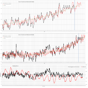
Obtaining the repetitive frequencies:
Using bandpass filters set to a bandwidth of f/150 (where f is the lower frequency of the BP filter) the filter is swept from 0.5year to 150 years looking for amplitude peaks.
As each peak is found the output from the filter is compared to the output of a cosine wave set to the filter output amplitude and to the centre frequency of the filter. The cosine wave is is then phase shifted to align the two waveforms.
This is repeated for as many peaks as are found in the HADCRUT3V record. Outputs from the BP filters that fall into likely TSI frequencies 10, 11, 12, 14, 21 years have their corresponding synthesized outputs nulled. 0.5 year output is also nulled.

TSI is phase shifted, amplitude modified, then it added or subtracted from sum of cosines (shift is +48 months and is subtracted). However from the start of records to a round 1900 a lower error is provided by adding the TSI!

The remaining synthesized outputs are then summed and modified by a multiplier constant (approx 2.69) set by minimising the error between synthesized and original HADCRUT.

No low frequency peaks were found that could fit the rise in temperature. The rise is obtained by curve fitting the HADCRUT data with a 3rd order polynomial:
y = 2.40389E-07x^3 - 1.34093E-03x^2 + 2.49320E+00x - 1.54550E+03

This is added into the synthesised data to provide the output data.

Because the reconstructed data is just the sum of cosines and TSI is relatively unimportant the data can be extended to the future in this case to about 2017.
The plots show 2011 to be cooling to mid year.

The following plots show the effects of
No TSI
TSI subtracted over whole period
TSI added until 1904 and then subtracted to current date

This is a plot of the frequencies and amplitudes used to obtain these plots. Disabled frequencies are shown as Zero amplitude. The output at 11 years represents TSI amplitude

Temperature http://www.cru.uea.ac.uk/cru/data/temperature/hadcrut3vgl.txt

band pass filter http://www.web-reg.de/bp_addin.html

Period years	amplitude	Phase
0.501165	0 - artificially set to zero	3977.413703
0.841963889	0.006750249	54.17800684
0.890040278	0.010820097	107.3740716
1.768375	0.006095148	63.60020753
1.937269444	0.006963534	46.86597827
1.992377604	0.005092903	5.83418163
2.038391667	0.004105465	40.65715905
2.107	0.004651939	23.05126836
2.264857778	0.007415539	29.18466231
2.3139375	0.009177612	69.3504266
2.541777778	0.006009001	23.33534812
2.675555556	0.007867544	52.76779754
2.745788889	0.004892064	10.93806807
2.87455	0.010417192	40.32797096
3.155483333	0.005246582	75.96412155
3.269194444	0.004667568	6.630682169
3.579391667	0.008309031	40.98807579
3.7625	0.008048213	9.685707583
3.775041667	0.008219473	29.02716352
3.990758333	0.005512257	55.81368265
4.703125	0.005653949	6.33244882
5.127033333	0.004919605	6.188780868
5.225694444	0.004829187	34.08701089
5.727361111	0.002816915	6.746840105
5.986555556	0.004839718	33.42814581
6.297588889	0.00394786	23.39636614
6.598588889	0.002294266	3.380314824
7.586036111	0.002836881	34.9110203
8.441377778	0.002737653	34.79750828
9.121972222	0.006211276	17.3232396
10.07848333	0 - artificially set to zero	6.888853744
TSI  WAVEFORM  set at 11 yrs	0.006495  THE TSI DATA	48 Months
11.45221389	0- artificially set to zero	28.41974504
12.38280556	0- artificially set to zero	22.96039729
14.79916667	0- artificially set to zero	16.96130996
21.17869444	0- artificially set to zero	23.39280935
35.88588889	0.001785871	10.89922244
64.19661111	0.002785835	16.71200197
64.21333333	0.002785776	4.134103705
2508.333333	1.56572E-06	0.302469618
2508.333333	1.56572E-06	0.30372208
2508.333333	1.56572E-06	0.462315105

Problems:

Just what is the filter capability of the BandPass excel plugin? A better version is required.

Need a better trend profile than the 3rd order polynomial

Bandpass filter is not good doeas not detect longer periods - insufficient length of data

=======

Yes - I know that with enough parameters you can match anything with a sum of sines. But this plot gives a reasonable match for 160 years so a few years into the future may also be well matched!

It should also be noted that there is an underlying trend (the polynomial == GHG forcing?) which is always positive. But there are many negative slopes and zero warming areas synthesized.