"With four parameters I can fit an elephant, and with five I can make him wiggle his trunk".
Attributed to von Neumann
Following on from comments The frequencies etc of the original plots have been tweaked.
Note no attribution of the frequencies found is offered!
Method:
All frequencies and TSI were removed leaving just the polynomial.
a frequency was fitted to the main humps of the HADCRUT data (59Years)
Amplitude and phase of this were matched to the temperature record
The residuals were obtained and a simple curve fit added.
This showed a period of about 100 years.
A Further frequency was fitted to this curve fit changing phase and amplitude and frequency to give a near zero curve fit too the residual
This produces a good low resolution fit.
An attempt was made then to further reduce the residuals by subtracting TSI:
This does not lower residuals significantly.
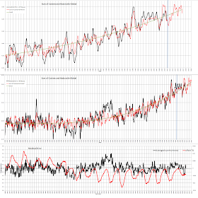
All frequencies are then re-instated and phase and freq of the 2 frequencies and TSI adjusted for minimum residuals:
A reasonable fit! Note that this is significantly better fit than the previous post around the twitch in 1945. This is because of the artificially input 60 year and 100 year waves.
 |
| The future |
None of the frequencies discovered produced the current rise so this has been trended with the following equation:
temp anom = 2.40389E-07(date)^3 - 1.34093E-03(date)^2 + 2.49320E+00(date) - 1.545547E+03
This trend produces the correct fit - It may be CO2 or something else. But I cannot see how a further cyclical parameter could produce the current rise.
Assuming that the trend is correct it produces the following prediction:
I DO NOT CLAIM THIS IS ACCURATE!!!!
However a very important point is that the trend is positive the whole of the time period. But the 2 major cycles 60 years and 100 years produce a substantially flat temperature from 2001 to 2023. During this period the trend continues rising and will add significantly to the 60 and 120 year cycles when they go positive.
This will allow "skeptics" 22 years of "I told you there was no warming" followed by an unfortunate, unexpected (to them) temperature rise.
TSI source still unknown but has little effect. The TSI has been extended to the future by splicing in data from 1900 a low level similar to this cycle?
=================================
All "sums" are done on monthly data and plots are filtered using a Hodrick Prescott filter (from the same source as the band pass filter) to remove high frequency components (HP filter gives a better end filter than moving average which has to terminate within 1/2 the averaging period from the end dates - in my opinion!)
The trend line is given by this polynomial:
y = 2.40389E-07x^3 - 1.34093E-03x^2 + 2.49320E+00x - 1.545547E+03
This trend fits the near horizontal 1800s and the increases since the 1960s
This could of course be a long period sine but if so then since the 1800s we have only gone perhaps half way through its cycle. this will only become visible in the next few decades if temperatures begin to decline.
The overall response with the increasing polynomial shows recent flatlining and even drops over the last year. The future prediction is for a decline for the next few years (the trend is still increasing remember!) as the 60y and 100y cycles go into a low period.
The frequency table (Frequency that would reconstruct the TSI data (9 years to 14 years + 21 years) has been artificially set to zero. The 2500 year data below is set to give 0 amplitude (no frequency found).
| Period years | amplitude | Offset months |
| 0.5012 | 0.023174092 | 6.60 |
| 0.8420 | 0.006750249 | 4.05 |
| 0.8900 | 0.010820097 | 0.59 |
| 1.7684 | 0.006095148 | 0.75 |
| 1.9373 | 0.006963534 | 2.85 |
| 1.9924 | 0.005092903 | 5.85 |
| 2.0384 | 0.004105465 | 9.20 |
| 2.1070 | 0.004651939 | 10.50 |
| 2.2649 | 0.007415539 | 10.35 |
| 2.3139 | 0.009177612 | 6.50 |
| 2.5418 | 0.006009001 | 4.50 |
| 2.6756 | 0.007867544 | 2.45 |
| 2.7458 | 0.004892064 | 4.65 |
| 2.8746 | 0.010417192 | 2.65 |
| 3.1555 | 0.005246582 | 0.56 |
| 3.2692 | 0.004667568 | 6.65 |
| 3.4699 | 0.004344144 | 9.34 |
| 3.5794 | 0.008309031 | 3.25 |
| 3.7750 | 0.008219473 | 3.90 |
| 3.9908 | 0.005512257 | 5.70 |
| 4.7031 | 0.005653949 | 6.25 |
| 5.1270 | 0.004919605 | 6.20 |
| 5.2257 | 0.004829187 | 9.05 |
| 5.7274 | 0.002816915 | 6.75 |
| 5.9866 | 0.004839718 | 2.05 |
| 6.2976 | 0.00394786 | 4.55 |
| 6.5986 | 0.002294266 | 3.50 |
| 7.5860 | 0.002836881 | 3.50 |
| 8.4414 | 0.002737653 | 3.35 |
| 10.0785 | 0 | 6.75 |
| 11 (TSI) | 0.014289 | 72.00 |
| 11.4522 | 0 | 3.25 |
| 12.3828 | 0 | 4.05 |
| 14.7992 | 0 | 4.35 |
| 21.1787 | 0 | 4.45 |
| 35.8859 | 0.001785871 | 4.65 |
| 59.4167 (not Found By filtering) | 0.041468451 | 3.35 |
| 103.5000 (not Found By filtering) | 0.017897547 | 101.05 |
| 110.1917 | 0 | 5.15 |
| 2508.3333 | 1.56572E-06 | 4.15 |
| 2508.3333 | 1.56572E-06 | 4.10 |
| 2508.3333 | 1.56572E-06 | 4.10 |


